This is my first ever blog post. So, it might have lot of mistakes and other problems. Feel free to share your opinions in the comment section. I hope, this post will help some or other in their path towards Deep learning and Neural Networks.
This post is about, Variational AutoEncoder and how we can make use of this wonderful idea of Autoencoders in Natural language processing. Here, I will go through the practical implementation of Variational Autoencoder in Tensorflow, based on Neural Variational Inference Document Model. There are many codes for Variational Autoencoder(VAE) available in Tensorflow, this is more or less like an extension of all these.
There are a lot of blogs, which described VAE in detail. So, I will be just referring to the core concepts and focus more on the implementation of this for NLP based on Neural Variational Inference Document Model. Generally, an AutoEncoder will reconstruct the input which we passed to it. This, ability of reconstructing an input (conventionally images), can easily be extended to reconstruct a document. Unlike, simple AutoEncoders which use, simple matrix multiplication to project the input to hidden state and use the transpose of the same matrix to reconstruct it back from the hidden state, here we use different matrices for input to hidden projection and hidden to output reconstruction. This can be viewed as, a Neural Network (Deep) , with encoder (input->hidden) and decoder(hidden->output).
VAE as Topic Model
Suppose you have trained a model with very large corpus of documents. We will discuss in detail shortly about, how we can feed a document as input to VAE. So, suppose your hidden layer is having 50 units . So, basically what we are trying to achieve or what we are achieving internally is projecting the document to 50 latent units. This can be interpreted as, mapping of documents to 50 topics. This has been neatly explained in Neural Variational Inference Document Model.
The part of a neural network, which maps the input to the hidden layer can be considered as a encoder. The encoder encodes the data or input into a latent vector. Suppose , you are having a huge corpus and you have created the vocabulary for the corpus.
- Let V be the vocabulary. (ie, the number of unique words in the whole corpus)
- Each document can represented a Bag of Words vector . That means , each document will be a vector of size V. Each index corresponding to a word in the vocabulary and if the word is present in the document, we will replace that index with count of the word in that document .
For a document d1, we can represent it as a vector. This will be of dimension V x 1.
Here 23, 45 represents the count of the words in the document .So, the next thing to do is map the input vector, to a hidden dimension, say 50. This can be achieved by matrix multiplication. Its up to us to think, how many layers deep, we need our encoder to be. Normally, 2 layer deep encoder works well. For, simplicity assume we have one layer, and we need a matrix ,to get a hidden state . This hidden vector is mapped back to the original document, by a matrix . Here, to calculate the probability of all words in vocab, a softmax function is using.
In the following figure, is the input vector (Bag of word vector), we need to find hidden layer or vector given (encoder) and we have to reconstruct it back from (decoder).
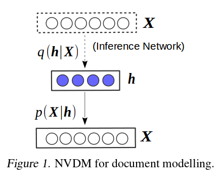
-
Why it is called Variational AutoEncoder?
There are wonderful tutorials out there, like Tutorial on Variational AutoEncoders. Here,
I will give a brief overview about what is happening under the hood.
Suppose we have a model with some hidden variables and some input . We may be
interested in inferring the hidden states from the input (that is, we want to know
what hidden states contributed to us seeing ). We can represent this idea using the
posterior distribution
By conditional probability,
But it is also true that,
(because = , the joint distribution of and )
So we can rearrange a bit:
In our model we have a graphical relationship between and . That is, we can infer which states caused , and we can generate more data from these hidden variables . We also have a prior distribution over our ’s, . This is often a Normal distribution. The problem is that term.
To get that marginal likelihood , we need to marginalize out the ’s. That is:
and the real issue is that the integral over could be computationally intractable.
That is, the space of is so large that we cannot integrate over it in a reasonable amount
of time. That means we cannot calculate our posterior distribution , since we can’t
calculate that denominator term, .
Note: The word
intractablehas a lot of meaning from the computational point of view and theoritical standpoint. A good discussion can be found over here.
One trick that’s used to combat this problem is Markov chain Monte Carlo, where the
posterior distribution is set up as the equilibrium distribution of a Markov chain. However,
this type of sampling method takes an extremely long time for a high-dimensional integral. The
more popular method right now is variationalinference.
In variational inference, we introduce an approximate posterior distribution to stand in for our true, intractable posterior. The notation for the approximate posterior is . Then, to make sure that our approximate posterior is actually a good stand-in for our true posterior, we optimize an objective to ensure that they’re close to one another in terms of a metric called ```Kullback-Leibler Divergence (KL Divergence)’’’. Think of this as a distance function for probability distributions: it measures how close two probability distributions, in this case and , are.
-
Objective Function
Lets say we have a document with words, such that . So, we basically wants to maximize the likelihood of these words in the output( while reconstructing). The objective function looks like:
That first term on the right hand side is the reconstruction loss; the second is the KL divergence. So that’s what’s going on in variational inference. That objective function is called the ‘variational lower bound’, the ‘expectation lower bound (ELBO’, the ‘lower bound on the marginal log likelihood’….It has so many names! There is a re-parameterisation trick used to sample the hidden states.
This is actually a common trick in statistics that’s only just caught on in the machine learning community. Say we have a very complicated distribution that we want to sample from. This distribution is so strangely shaped that standard sampling tricks won’t help us. To combat this problem, we sample from a simpler distribution and then transform the samples to look like the distribution we actually wanted to sample from.Here’s an example:
Say we want to sample from a distribution (yes, this is actually easy to sample from, but it’s a good example because we can see it in our mind’s eye). Pretend this distribution is hard to sample from. It’s easy to sample from a distribution. We generate samples . Let’s say we get samples.
Then to transform these samples to what we really wanted (a sample) we do a linear transformation:
This transforms our sample from a distribution to a distribution. That relationship is possible because the Normal distribution belongs to the location-scale family. Distributions more complicated that that could require nonlinear transformations. Please have a look at the referred link for more details.
-
Implementation in Tensorflow
The implementation of the code is in Tensorflow. The full code is available here. I will go through some key aspects of implementing the Variational Auto Encoder, for Language Processing. The dataset using here is 20 news group dataset. In practice, instead of going over each document separatey, we will feed a batch of data to the model for training. This is more effective in practice, due to the computational complexity in training a Deep Neural Network.
The main file to run is defined as main.py in the repo. In main.py, we load necessary functions and packages, useful for preprocessing and loading the data.
from text_loader_utils import TextLoader
from variational_model import NVDM

######## flags are originally defined in the code #########

def main(_):
  print(flags.FLAGS.__flags)

  from sklearn.datasets import fetch_20newsgroups
  twenty_train = fetch_20newsgroups(subset='train')
  data_ = twenty_train.data
  print "Download 20 news group data completed"

  data_loader = TextLoader(data_ , min_count = 25)
  n_samples = len(data_)
  total_batch = n_samples/FLAGS.batch_size
  print "Data loader has been instantiated"
  gpu_opts = tf.GPUOptions(per_process_gpu_memory_fraction=0.9)
  with tf.Session(config=tf.ConfigProto(gpu_options=gpu_opts)) as sess:

    model = NVDM(sess ,  len(data_loader.vocab), FLAGS.hidden_dim,
                         FLAGS.encoder_hidden_dim ,
                         transfer_fct=tf.nn.tanh ,
                         output_activation=tf.nn.softmax,
                         batch_size=FLAGS.batch_size,
                         initializer=xavier_init , dataset = FLAGS.dataset ,
                         decay_rate = FLAGS.decay_rate ,
                         decay_step = FLAGS.decay_step ,
                         learning_rate = FLAGS.learning_rate ,
                         checkpoint_dir = FLAGS.checkpoint_dir )


    model.start_the_model(FLAGS , data_loader)
The TextLoader class, plays the role of pre-processor and vocab creator. If you are familiar with
numpy, creating a Bag of word matrix for the entire dataset ( here, approx 11k documents ) is not
feasible from the memory point of view. So, we are creating an iterator, which in real time will iterate
and create Bag of words matrix, to feed to the network. This is instantiated in data_loader, and we
are passing it to the model. gpu_options is configurable, and it is not necessary to set it to 0.9,
as Tensorflow is greedy in memory consumption. Further parameters will be discussed on the go. The hidden_dim is 50 and the encoder_hidden_dim is [500, 500]. So, the encoder is 2-layer deep here.
def start_the_model(self , FLAGS , data_loader):

        self._train()

        print "Try loading previous models if any"
        self.load(self.checkpoint_dir)

        start_iter = self.step.eval()
        print "Start_iter" , start_iter
        for epoch in range(start_iter , start_iter + FLAGS.training_epochs):
            batch_data = data_loader.get_batch(FLAGS.batch_size)
            loss_sum = 0.
            kld_sum = 0.
            # Loop over all batches
            batch_id = 0
            for batch_ in batch_data:

                batch_id += 1
                collected_data = [chunks for chunks in batch_]
                batch_xs , mask_xs , _  = data_loader._bag_of_words(collected_data)
                _ , total_cost , recons_loss_ , kld , summary_str     = self.partial_fit(batch_xs,
                                                                          batch_xs.shape[0], mask_xs)
                word_count = np.sum(mask_xs)
                batch_loss = np.sum(total_cost)/word_count
                loss_sum += batch_loss
                kld_sum += np.sum(kld)

                print (" Epoch {} Batch Id {} , Loss {} , Kld is {}  ".format(epoch+1 , batch_id , batch_loss, np.sum(kld)))

            print_ppx = loss_sum
            print_kld = kld_sum/batch_id

            print('| Epoch train: {:d} |'.format(epoch+1),
                   '| Perplexity: {:.5f}'.format(print_ppx),
                   '| KLD: {:.5}'.format(print_kld))


            if epoch % FLAGS.save_step == 0:
              self.save(self.checkpoint_dir, epoch
Few things to note here, it is just a wrapper for training. The batch_data is an iterator of data in
batches, which needs to be called everytime once an epoch is over. Because, it will run out of data,
as it it iterates over each batch in every epoch. batch_xs, is a matrix of Bag of word vector of
documents. Normally, batch_xs is of shape , where 100 is the batch_size. mask_xs
is mask, which means wherever the index of batch_xs is not 0, we will have 1, over that
index in mask_xs. In simple words, batch_xs hold the count of words in a document, where as
mask_xs, holds a value of 1 in the corresponding index, just to indicate the presence of the word.
If you are familar with Tensorflow, we have to feed the necessary data to the corresponding place holders.
This is happened in partial_fit method. Note, we are passing batch_xs.shape[0], because,
suppose we have batch of 100 documents and after pre-processing, we will be having only 98. So, the value
of batch after pre-processing might remain same or vary, from the original batch_size.
Lets have a look at each function one by one. This might be boring to those who are super familiar with Tensorflow. But, those who wants to know more in a practical point of view, this might be useful. Inside the NVDM class, we have different functions.
The create_network, will call _initialize_weights method, which is responsible for buliding the Weights and biases, for both encoder and decoder. It has been written, in such a way that, it will accept any layer of encoder_hidden_dim. Here, it is [500, 500], so we will have self.Weights_encoder a dictionary, with keys as W_1 ,W_2, 'out_mean' and 'out_log_sigma', which is useful in finding a new sample as explained in re-parameterization trick. ‘self._encoder_network, is easy to understand, it has basic matrix multiplication with a non-linearity on the top, except at places where out_mean and out_log_sigma is used.
self.z_mean, self.z_log_sigma_sq = self._encoder_network(self.Weights_encoder, self.Biases_encoder)

# Draw one sample z from Gaussian distribution
eps = tf.random_normal((self.dynamic_batch_size, self.hidden_dim), 0, 1,
                       dtype=tf.float32)
# z = mu + sigma*epsilon ( Re-parameterization)
self.z = tf.add(self.z_mean,
                tf.mul(tf.exp(self.z_log_sigma_sq), eps))
This self.z sample, is used to re-construct the document vector (batch of document vector in practice). This is happening inside self._generator_network.
x_reconstr_mean = tf.add(-1*(tf.matmul(self.z, weights['out_mean'])),
                                     biases['out_mean'])
The above equation is equivalent to Eq.24 in here. There, the equation is shown on the basis of each word and represents, the One-hot_K vector associated with each word in the vocab. Note, this one hot vector for words are different from Bag of words of document.
So, we had all components necessary to calculate the loss function. In the Objective section, I have pointed out the loss function. This can be viewed as maximizing the log-likelihood of words present in each document and minimzing the KL divergence, between the distributions.
is the number of documents and is the number of words (not the count of all words), present in each document. This will vary with document. To achieve this in fast matrix operation, after calculating the ‘'’softmax’’’, we multiply the resultant matrix with the mask_xs ( which has 1 at the index where words are present and 0 if words are absent), matrix and then do the summation.
, is the matrix we have in self.Weights_generator['out_mean']. The interesting thing is once, we train the model, this , acts as the embedding matrix.
The loss function are defined inside _create_loss_optimizer.
logits = tf.log(tf.nn.softmax(self.X_reconstruction_mean)+0.0001)
self.reconstr_loss  = -tf.reduce_sum(tf.mul(logits, self.X), 1)

self.kld = -0.5 * tf.reduce_sum(1 - tf.square(self.z_mean) + 2 * self.z_log_sigma_sq - tf.exp(2 * self.z_log_sigma_sq), 1)

self.cost = self.reconstr_loss + self.kld   # average over batch
# Use ADAM optimizer

self.optimizer = tf.train.AdamOptimizer(learning_rate=self.learning_rate).minimize(self.cost , global_step=self.step)
The equations for KL divergence is quite common and you can find it everywhere. In the original paper, author used alternative update. But, i don’t think that is necessary. Here, we sum up the encoder loss and decoder loss. In the code, generator, stands for decoder. We use, AdamOptimizer for training. So, this is what is happening under the hood and the main wrapper fuunction is _partial_fit.
def partial_fit(self, X , dynamic_batch_size , MASK):


        opt, cost , recons_loss , kld   = self.sess.run((self.optimizer, self.cost , self.reconstr_loss , self.kld ),
                                  feed_dict={self.X: X , self.dynamic_batch_size:dynamic_batch_size,
                                            self.MASK:MASK})
return opt , cost , recons_loss , kld -
A note about non-linear functions
In the paper, author has used
ReLU, activation functions. But, don’t use it. I was gettingnanvalues after 2 iterations. The reason, I am thinking is our document vector has some large values like 123, 371 , which are the count of words in the document. As, ReLU is doing max(0, N), this might be the reason. Usetanh. It will works fine. If you still want to use,ReLU, normalize your Bag of word matrix each time before passing to the model.
-
Evaluation of the model
I have ran the model in p2.xlarge in AWS, for 1000 iterations and it took around 6 hrs. The model can be
found inside the github repo. I have used the embedding matrix to find similar words and results are
very good. I have uploaded a ipython notebook model_evaluation.ipynb, which shows how to use the
model to extract the embedding matrix and find similar words.
Here are examples of some words
jesus
[('jesus', 0.99999988),
 ('christ', 0.85499293),
 ('christian', 0.77007663),
 ('christians', 0.75781548),
 ('bible', 0.75542903),
 ('heaven', 0.74329948),
 ('god', 0.73894531),
 ('sin', 0.72564238),
 ('follow', 0.71326089),
 ('faith', 0.69616199)]
scientist
[('scientist', 1.0),
 ('hypothesis', 0.79111576),
 ('mathematics', 0.7701571),
 ('empirical', 0.74546576),
 ('experiment', 0.74009466),
 ('scientists', 0.73293155),
 ('observations', 0.72646093),
 ('psychology', 0.72322875),
 ('homeopathy', 0.7231313),
 ('methodology', 0.71882892)]
football
[('football', 1.0000001),
 ('stadium', 0.85528636),
 ('basketball', 0.8517698),
 ('philly', 0.83852005),
 ('mlb', 0.83592558),
 ('robbie', 0.83328015),
 ('anyways', 0.82795608),
 ('seats', 0.82188618),
 ('miami', 0.82166839),
 ('champs', 0.81938583)]
-
Similar Documents
The hidden dimensions for each document can be used to calculate similar documents. The function used here is mentioned in the notebook. This is very useful in information retrieving tasks.
-
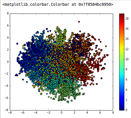
Clustering
The same model, with the hidden representaions can be used for clustering. The following
figure has been generated on 20 news group dataset, by projecting each 50 dimension hidden
state of every document into tsne . The plot looks very promising .
I would like to thank the author’s of the paper, for giving a intuitive idea of VAE in NLP point of view. And I would like to thank my friend Carolyn Augusta, (explanation about Variational Bayes and Re-parameterization was from her courtesy). I hope, she will be having a detailed writing about the Variational Bayes soon. Please do point out the mistakes, if you found any.